فیلتر کردن سلول های مرق شده (ادغام شده) و عدم نمایش blank در اکسل
How To Filter All Related Data From Merged Cells In Excel?
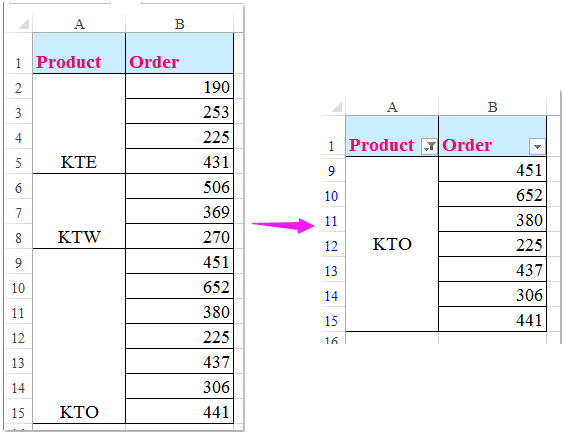
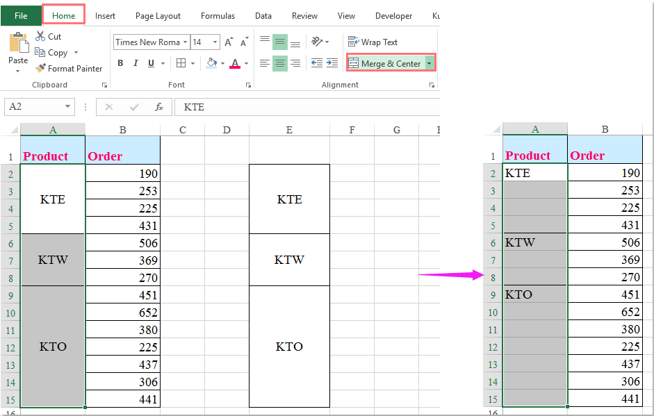
Supposing there is a column of merged cells in your data range, and now, you need to filter this column with merged cells to show all the rows which are related with each merged cell as following screenshots shown. In excel, the Filter feature allows you to filter only the first item which associated with the merged cells, in this article, I will talk about how to filter all related data from merged cells in Excel?
Filter all related data from merged cells in Excel
|
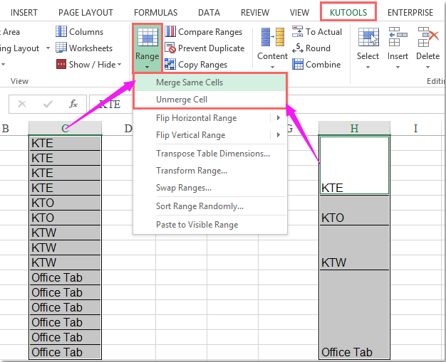
Merge or unmerge same cells in columns:
Kutools for Excel’s Merge / Unmerge Same Cells utility can help you merge and unmerge adjacent rows which have same value into one cell with only one click.
Kutools for Excel: with more than 200 handy Excel add-ins, free to try with no limitation in 60 days. Download and free trial Now! |
Filter All Related Data From Merged Cells In Excel

To solve this job, you need to do following operations step by step.
1. Copy your merged cells data to other blank column in order to keep the original merged cell formatting.
2. Select your original merged cell (A2:A15), and then click Home > Merged & Center to cancel the merged cells, see screenshots:
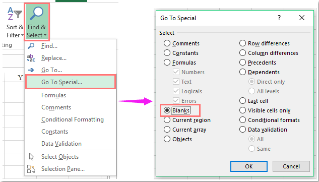
3. Keep the selection status of A2: A15, and then go to Home tab, and click Find & Select > Go To Special, in the Go To Specialdialog box, select Blanks option under Select section,see screenshot:
4. All the blank cells have been selected, then type = and press Up arrow key on keyboard, and then press Ctrl + Enter keys to fill all the selected blank cells with the value above, see screenshot:
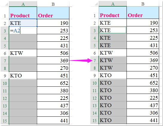
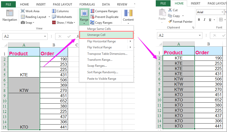
| Tips: If you have Kutools for Excel, with its Unmerge Cell utility, you can unmerge the merged cells and copy down the duplicate values at one click. |
 |
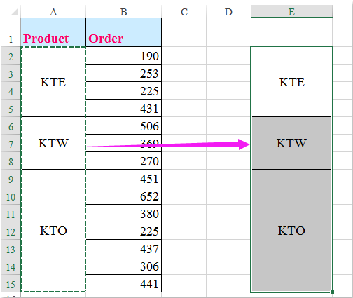
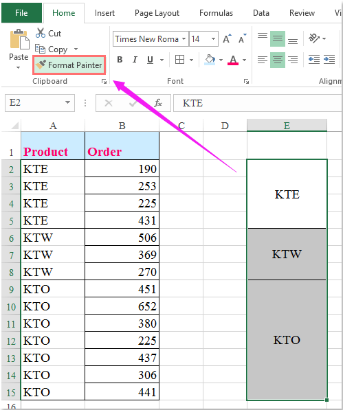
5. Then you need to apply the formatting of your pasted merged cells in step 1, select the merged cells E2:E15, and click Home >Format Painter, see screenshot:
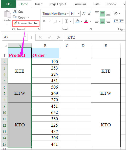
6. And then drag the Format Painter to fill from A2 to A15 to apply the original merged formatting to this range.
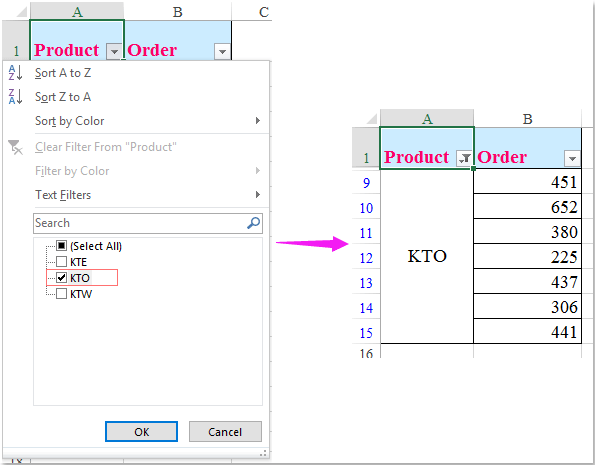
7. At last, you can apply the Filter function to filter the item that you want, please click Data > Filter, and choose your needed filter criteria, click OK to filter the merged cells with all their related data, see screenshot:
 دانلود موزیک روز کامپیوتر جوک و sms اس ام اس مطالب جالب